Helicopter money part III: economic stimulus

What is helicopter money (HM)¹ supposed to accomplish? Advocates of HM believe that HM acts as a stimulus which increases the level of economic activity. In this post, I construct a simple model and show in detail how it works. The steady state economy – an economy with a constant aggregate nominal income and expenditure per time – is described first. Next, the effect of reduced spending and income of the agents is illustrated. And then it is discussed how the economy can be returned to its previous steady state of spending.

What are the assumptions behind the model? And what is the scope of this post?

• The economy is closed, there are no inflows from or outflows to the “rest of the world”
• There is one single currency
• Only nominal amounts and flows of money are considered in this post.

The effects of stimulus on prices and exchange rates will be discussed in later posts.

Easy numerical examples are used throughout this blog post. As I wrote before, this avoids the hidden inconsistencies that many words-only economic commentaries suffer from. The reader can check the logic of the model and expand it further for his own use. This should make it a powerful analytic tool for economists. I am planning to frequently use this model for further research, to answer questions regarding balance of payments and transfers between economic classes².

 

Keeping track of ‘circular flows’ of money: the money flow matrix

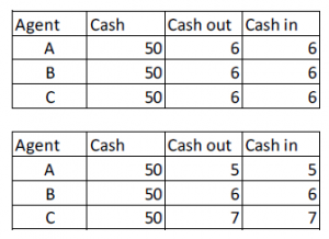
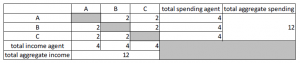
Suppose there are three agents³: A, B, and C. Each has €50 in physical cash. There is no banking system in the model of this post. In aggregate, there is a fixed amount of cash⁴ equal to €150. Assume that in the steady state (SS)⁵ each agent spends⁶ €6 per month on average (€72/year). There are many “microscopic” ways to realize this economy, for example:

The income of each agent depends on the expenditure of the other two agents. The idea that money does not disappear when it is spent, but becomes someone else’s income, is known as circular flow. Although this is an intuitive concept, circular flow is hard to quantify. Pictures full of arrows between sectors⁷ are almost impossible to use for thorough numerical reasoning.

To keep track of how the money flows between agents, I am going to use something I call a money flow matrix (MFM). This is a visualization method that keeps track of who the agents give money to (the horizontal rows) and whom they receive money from (the vertical columns). The amounts in the MFM are expressed in currency per time unit.

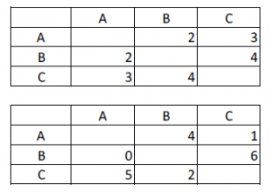
To keep things as simple as possible, we will work with the steady state (SS) economy of figure 1a. To simplify further, the agents’ income from the others is divided evenly at €3/month per agent:

 

A shock disturbs the steady state

For some reason, the SS gets disturbed. Agent A reduces his nominal spending by 2€/month. There can be multiple reasons for this. For example: the prices of the goods and services that B and C sell to A fall (so that A buys the same things as before, but pay less for it), or A wants to save more of his income⁸.

The MFM when agents B and C spend their usual amount of money is shown at the bottom of figure 4.

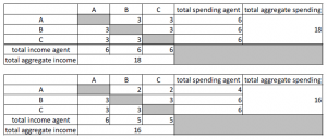
Agent A ends up with €50 + €6 – €4 = €52 after this month. B and C each only have €49 (=€50 + €5 – €6) left at the end of the month. There has been a shift of money between the agents. More importantly, the “economic activity”, i.e. the total aggregate nominal amount of spending and income has decreased from €18/month to €16/month.

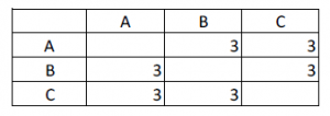
Now imagine that B and C react to their loss of income by also reducing spending to €4/month. The MFM for this new situation looks as follows:

In summary: although the total amount of money in the economy is constant at €150, the monthly nominal spending and income has decreased by 33%.

Note that for each and every month, the sum of spending is equal to the sum of income. This is immediately visible from the structure of the MFM. What is different is the behavior (i.e., the spending decisions) of the agents from one month to the next.

 

Adding the government

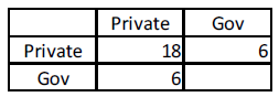
We now introduce the government in the model. To keep our previous examples, the government is added as an extra agent in the MFM.

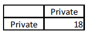
In what follows, agents A, B and C are aggregated into one single “effective agent” that we call Private (i.e. the private sector, as opposed to the government). One practical remark before we continue: so far, the diagonal elements of the money flow matrices have always been greyed out. It would not make sense for an individual agent to pay himself money. But when the agents are aggregates, the money that is spent “within” the agent (i.e. between the constituent parts of the effective agent) should be accounted for in the MFM.

Let’s say that the government levies taxes equal to one third of the intra-private sector income⁹. Suppose further that the government runs a balanced budget in the steady state. This means that the government’s expenditure (by definition to the Private sector, as our model world is closed) is equal to what it taxes. By taxing and spending the government redistributes money within the private sector. This intra-Private distribution is not relevant for the rest of this post.

Our example including the government (Gov) is summarized in the MFM of figure 7.

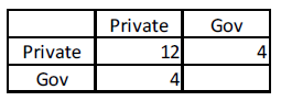
Now suppose that the intra-Private sector spending reduces from €18/month to €12/month, like in figure 5. The government immediately adjusts spending to the falling tax receipts.

What can the government do to return intra-Private spending and income to its previous level?

Maybe the problem is that private agents are prevented from doing business. For example: heavy snowfall blocks roads, so people cannot access shops and businesses. In this case, the government could clear the roads. Or it could be that agents don’t spend money at bars and airports due to terrorism concerns. Then the government should improve safety.

The government could also try and force the agents to spend more. In reality, this would be hard to do. Would it jail those who do not spend more? And how would compliance be verified? When prices have dropped, price controls could be imposed to increase prices and wages¹⁰. A variation on this theme is when it is judged that the spending reduction is a consequence of falling asset prices. The government could force fund managers to buy at higher prices. Some believe the resulting wealth effect would tempt agents to increase spending.

The remainder of this post focusses on another policy. The government stimulates the economy by spending more money (compared to the previous time period). This would raise the income of the private agents. It is then hoped that they will increase their intra-Private spending.

 

Stimulus and the multiplier

Let’s say that the money flows in the economy during month 0 are described by the MFM in figure 8. The next month, the Government spends €12/month to Private¹¹. Debt and banking is out of the scope of this article, so let’s say that Gov printed the money¹².

The government expenditure is a so-called fiscal stimulus. The stimulus can have many forms: unemployment benefits, wages of state employees, payments for services of companies, “true” helicopter money (i.e. unconditionally distributed to the people)…

The hope is that by raising the income of the private sector, the total spending of the economy will grow. This is called the multiplier effect of the stimulus.

What counts as stimulus? I define the stimulus as the government expenditure above the Gov expenditure of some hypothetical baseline in a certain period of time. The reason for this is to avoid labeling all government expenditure stimulus.

The baseline of our example is the depressed state of figure 8. Without stimulus, the government would spend €4. When it spends €12 instead, this means that it injects a €8 stimulus into the economy.

When the multiplier m is 1, the total spending (of Private + Gov) grows by the exact amount of the stimulus. This would be the case of people put helicopter money under their mattress and don’t change their spending compared to figure 8.

When the multiplier m < 1, Private spending decreases compared to the baseline.

However, it is likely that the private agents will be more inclined to spend money because their (aggregate) income rises. The private sector can increase spending by employing more people, by buying more stuff, by raising wages… In that case, m > 1.

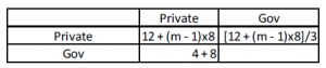
Note that when m = 4, the stimulus would pay for itself within the month that it was spent (see figure 9). The tax revenues (assumed to be 1/3 of intra-Private income) would be €12, the same amount that Gov spends on Private, thus balancing the budget. Note that with such a high multiplier, the nominal spending in the economy far exceeds the previous steady state of figure 7.

 

Predicting the effect of the stimulus

It should be clear that the model in this article can describe what happens in consistent terms. Predicting the outcome of the stimulus however depends on the behavior of the private agents. Economists can measure the multiplier m in historical data¹³ but cannot treat it as a constant for predicting the effect of future policy. The economy is a complex system where a similar “impulse” (Gov stimulus) will not always result in a similar outcome.

Some logical thinking does lead to the conclusion that stimulus that puts money in the pocket of the poor will increase spending. It is likely they will not keep the extra income in their wallet, but spend it on basic goods (food, rent, clothes…). In the words of Keynes, they have a high propensity to consume. When richer private agents do not cut spending, the aggregate m will be higher than one.

The size of the multiplier depends on counterfactuals. There is only one unique economy in reality, with no possibility to go back to the start and play another scenario. This makes it ideal for economists – a notoriously quarrelsome bunch – to disagree with one another.

To illustrate the dependence of the multiplier on hypothetical scenarios and its time dependence, consider the following.

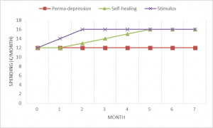
Let’s say the stimulus of €8 is spent during one month in the depressed economy of figure 8. The multiplier for this stimulus is derived based on two alternative scenarios. In the “perma-depression” (PD) scenario, intra-Private spending is assumed to remain at €12/month indefinitely. In the “self-healing” (SH) scenario, intra-Private spending picks up without government intervention, albeit at a slower pace compared to the stimulus scenario. The monthly intra-Private spending for these three scenarios is given in figure 10.

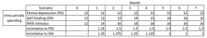
The scenarios of figure 10 are plotted in figure 11.

As shown in figure 9, the multiplier m can be calculated by this equation:

Baseline intra-Private spending (in time period) + (m(time period) – 1) x stimulus = intra-Private spending with stimulus (in time period)

So the multiplier in month 2 (the month after the stimulus) under the SH baseline scenario is given by: 13€ + (m-1)x8€ = 16€ => m = 1.375

What if the time period is measured per half year instead of per month?

The multiplier for months 1 to 6 in figure 10 under the SH baseline is: 86€¹⁴ + (m-1)x8€ = 94€¹⁵ => m = 2.

The PD scenario shows the importance of defining a cut-off time, after which the stimulus effects are neglected. The 6-month multiplier of the stimulus with the perma-depression baseline is 3.75¹⁶, while the 1 year multiplier is 6.75¹⁷.

As a final note on the time dependence of the multiplier, there can be an increase of the intra-Private spending already before the stimulus is spent. When companies hire lobbyists to get the new government contracts, when they train new workers or buy new equipment part in anticipation of the stimulus package, private spending rises in the months prior to the extra government spending.

 

Summary

• This post described the money flow matrix, a tool for analyzing money flows in time
• Total income per time unit is ALWAYS equal to total spending in the time unit
• Spending decisions make income different from one time period to the next
• Economists suck at analyzing circular flow/stimulus/multipliers
• The effect of government stimulus depends on the actions of the private sector
• The multiplier effect is hard to determine because it depends on counterfactuals
• The multiplier can only be properly discussed when the baseline scenario and time frame are specified
• This article only looked at nominal flows in one currency. Banking, inflation, FX effects… are all out of scope the current post.

 

1. Earlier posts in this series looked at the balance sheet implications of helicopter money and its political aspects.
2. Balance sheets and the money flow matrix are the two conceptual pillars that support the technical analyses in my upcoming book.
3. ’Agent’ is used as a general term for economic entities. The agents can be individuals, businesses, NGOs, municipalities…
4. As anyone who has read my previous posts on QE and helicopter money should know, banks can make and destroy money in accounts. This is a long post, so I decided not to add the complication of credit.
5. ’Steady state’ means that there is a dynamic equilibrium. Although money changes hands, the average stock and flow of cash per agent stays the same.
6. This post only looks at the money, I am not interested in what the money is spend on: paying for consumer goods, wages, rent…
7. Search for circular flow on Google Images.
8. For example to prepare for future income loss (prospect of retirement, unemployment…) or to make up for a drop in the value of A’s assets (e.g. when housing prices fall)
9. For example by an income tax on wages and a tax on business revenues, like VAT.
10. This is a counterintuitive concept, as the goal of price controls is usually to lower prices.
11. The reason I choose €12/month is that the total SS income of Private was €24/month, see figure 7. Assuming a depressed intra-Private spending of €12/month (figure 8), the increase in Gov spending would raise total Private income to its high SS level.
12. Net of taxes.
13. This is a fancy way of describing parameter fitting.
14. 12 + 13 + 14 + 15 + 16 + 16 = 86
15. 14 + 16 + 16 + 16 + 16+ 16 = 94
16. (6×12) + (m-1)x8 = 94
17. 12×12 + (m-1)x8 = 14 + (11×16)